NON-PARAMETRIC ANALYSES:
DISTRIBUTION FREE, BUT NOT ASSUMPTION FREE
Poster Presentation
Mariska Burger - Senior Biostatistician - OCS Life Sciences
Introduction
Many conventional statistical methods require the assumption that your data are normally distributed. When these assumptions are violated, such methods might fail and might lead to wrong conclusions.
What if your data is not normally distributed and you have already exhausted all meaningful data transformations and investigated outliers and you have no other option but to analyze your data using non-parametric statistical methods?
What can you conclude from using for example the Wilcoxon Mann-Whitney (WMW) test and are there assumptions you need to verify before making any conclusions?
Non-parametric tests may be distribution free, but not assumption free. A lot of publications, researchers and statisticians interpret the WMW p-value blindly as a test for difference in medians without checking assumptions. O’Brien and Castelloe (2006) noted: “Even worthy statistics books (and knowledgeable statisticians!) state that the WMW test compares two medians, but this is only true in the rarest of cases in which population distributions of two groups are merely shifted versions of each other (i.e., differing only in location, and not shape or scale).” [1] We will explore the WMW test and some other non-parametric tests with their assumptions and introduce bootstrapping as an alternative
Wilcoxon Mann-Whitney Test [2]
The WMW test compares the whole distribution between two groups and the hypothesis being tested can be written as follow:


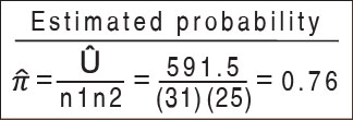
What can we conclude? There is a significant difference in Variable Z between Treatment X and Y or otherwise stated that the probability that a random observation drawn from Treatment X has a bigger value for Variable Z than a random observation drawn from Treatment Y is not 50% (76%).
In example 2, we demonstrate that two distributions with different median values, 9 for Treatment A and 29 for Treatment B, can have a non-significant WMW p-value (>0.999).

As can be seen from the two examples above, the value of the WMW test statistic compares how two sets of observations are distributed relative to one another and does not compare any central tendency parameter (eg. median).
Under what assumptions can the WMW test then be interpreted as a difference between the medians, or as a “pure shift”?
The following hypothesis of the WMW is true ONLY if it is assumed that the two populations being compared have identical shapes (same variances, same skewness etc.) and that the only potential difference is the location.

If the “pure shift” assumption holds then δ will be an estimate for the difference between medians, but also between the 5th percentiles or the 95th percentiles etc.
Other Non-parametric Tests
• The Hodges-Lehmann estimate can estimate the difference in medians between two groups, but only if the assumption of symmetrical data around the median within groups hold. If this assumption does not hold the Hodges-Lehmann estimate the median difference rather than the difference in medians [3].
• The Mood’s Median test tests the equality of medians from two or more populations. Although the Mood’s median test does not require normally distributed data it does require that the data from each population is an independent random sample and the population distributions have the same shape.
• Quantile regression makes no assumptions about the distribution of the residuals, is more robust to the existence of outliers, allows you to control for covariates, but has the major drawback that it needs sufficient data and is computationally intensive [3].
Bootstrapping [4]
Alternatively, bootstrapping can be used to calculate standard errors and confidence intervals without knowing the type of distribution from which the sample was drawn. It is a data-based simulation method to assign measures of accuracy to statistical estimates. The method of bootstrapping was first introduced by Efron around 1993 as a method to derive the estimate of standard error of an arbitrary estimator.
The use of the term 'bootstrap' comes from the phrase “To pull oneself up by one's bootstraps”, generally interpreted as succeeding in spite of limited resources.
The only assumption for bootstrapping is that the data are a random sample. The bootstrap simulates what would happen if repeated samples of the population could be taken by taking repeated samples of the data available. Empirical research suggests that best results are obtained when the repeated samples are the same size as the original sample and when the samples are drawn with replacement.
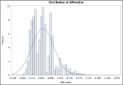
For the data from Example 1, we can obtain the 95% confidence interval for the difference in medians between Treatment X and Treatment Y using bootstrapping:

What is the BCa method?
It is an improved method of calculating confidence intervals addressing:
1. Bias - any systematic under or over estimation of our sample statistic when calculated using bootstrap resampling.
2. Acceleration - rate of change of the standard error of the estimate of our sample statistic with respect to the true value of the statistic (calculated using jackknifing).


What can we conclude? The 95% confidence interval for difference in medians of Variable Z between Treatment X and Treatment Y is (-0.076 ; 0.101) and since the confidence interval contains zero, we can conclude that there is no statistical significant difference.
Just like in a normal non-bootstrap setting where the parametric estimate accepts the possibility that a sample can be non-representative by random occurrence, the bootstrap also depends on the sample being a good representation of the whole population from which you are sampling.
Bootstrap diagnostics can be used to examine whether conclusions depend heavily on any single observation. Sometimes we also observe an “extreme” bootstrap sample and in order to avoid this chance occurrence of an extreme bootstrap sample to unduly influence the bootstrap confidence interval, one can re-calculate the confidence interval excluding these extreme bootstrap samples.
Conclusion
• The WMW test compares the whole distribution of two groups under the general hypothesis. Only under the “pure shift” alternative hypothesis, the WMW test can be interpreted as a test for the difference between medians.
• Other available non-parametric tests, like the Hodges-Lehmann estimate and the Mood’s mediantest require certain assumptions to hold. And, although quantile regression has some advantages it has the major draw back that it needs large sample sizes to be accurate.
• The bootstrap data-based simulation method is a relatively robust method to assign accuracy to any statistical estimate, since it does not make any assumptions about the distribution of the population from which the sample was drawn.
Remember, non-parametric statistics might be distribution free, but they are not assumption free and I suggest that you always plot your data in order to verify the underlying assumptions before making any conclusions.
Acknowledgements and References
I would like to thank all my colleagues who took part in fruitful article discussions, validated my results, designed and reviewed my poster.
1. O'Brien, R. G. and Castelloe, J. M. (2006), Proceedings of the Thirty-first Annual SAS Users Group International Conference, Paper 209-31. Cary, NC: SAS Institute Inc;. Exploiting the Link between the Wilcoxon–Mann–Whitney Test and a Simple Odds Statistic
2. George W. Divine, H. James Norton, Anna E. Barón & Elizabeth JuarezColunga (2018) The Wilcoxon–Mann–Whitney Procedure Fails as a Test of Medians, The American Statistician, 72:3, 278-286, DOI: 10.1080/00031305.2017.1305291
3. Staffa SJ, Zurakowski D. Calculation of Confidence Intervals for Differences in Medians Between Groups and Comparison of Methods. Anesth Analg. 2020 Feb;130(2):542-546. doi: 10.1213/ANE.0000000000004535. PMID: 31725019.
4.Barker, Nancy G. “A Practical Introduction to the Bootstrap Using the SAS System.” (2005).


